contagion

Summary

contagion is a network epidemic simulation package designed to make implementing complex node immunization policies easier. A selection of its features:

• heuristic-based immunization algorithms,
• partial immunity,
• time-varying transmission rates,
• tracking for symptom development,
• different testing procedures, whose rates can be tuned separately for symptomatic/asymptomatic nodes,
• temporary immunity, whose duration may vary based on how the immunity was conferred,
• delayed immunization, and more.

Example Usage

We provide a few brief use cases. For illustrative purposes, we focus on plotting-related methods; a more detailed overview of functionality is available in the documentation. Here, all examples use random contact networks generated by the Barabási–Albert preferential attachment procedure.

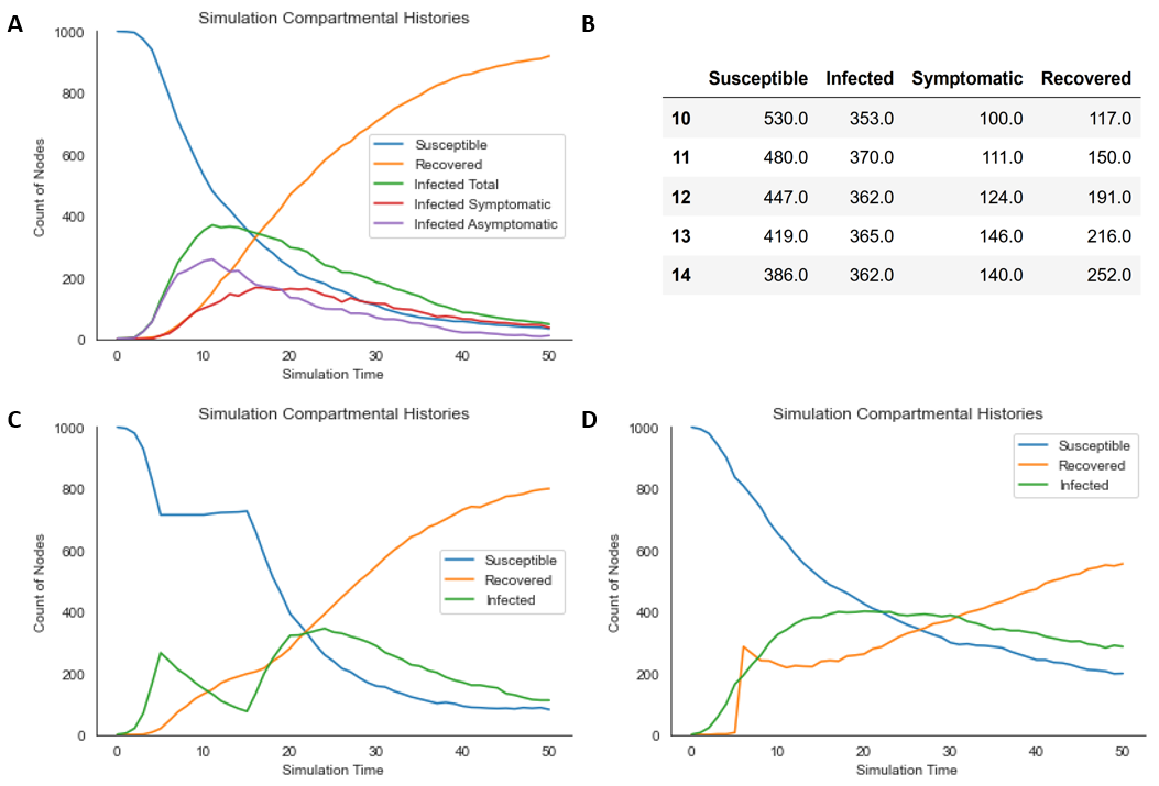
We begin with a basic simulation, whereby the contagion has a relatively aggressive transmission rate (beta = 0.2), an average recovery time of 10 time-steps (gamma = 0.1), and an average time-to-symptom-development of 5 time-steps (gamma = 0.2):

 network = contagion.ContactNetwork(
     nx.barabasi_albert_graph(1000, 5))

 sim = contagion.Contagion(
     network = network,
     beta = 0.2,
     gamma = 0.1,
     track_symptomatic = True,
     psi = 0.2)

 sim.plot_simulation(steps = 50)

The resultant rendering is displayed in Figure 1A. Practical details, including compartmental histories, are recorded as simulation attributes, which can be retrieved afterward (Figure 1B):

 df = pd.DataFrame(data = {
     "Susceptible": sim.Su_hist,
     "Infected": sim.In_hist,
     "Symptomatic": sim.Sy_hist,
     "Recovered": sim.Re_hist})
 df[10:15]

Our second example illustrates time-varying transmission rates, which may be representative of uniformly-adopted non-pharmaceutical interventions or seasonal dynamics, and a small probability of immunity loss after recovery (omega = 0.01). The transmission rate (beta) is 0.3 for the first 5 time-steps, 0 for the next 10, and 0.3 again for the remainder of the simulation, resulting in two distinct infection peaks:

 network = contagion.ContactNetwork(
     nx.barabasi_albert_graph(1000, 5))

 sim = contagion.Contagion(
     network = network,
     beta = [0.3]*5+[0]*10+[0.3],
     omega = 0.01,
     gamma = 0.1)

 sim.plot_simulation(steps = 50)

The resultant rendering is displayed in Figure 1C.

Finally, we introduce some of contagion’s node immunization functionality. After 5 simulation steps, we immunize half the network according to eigenvector centrality, using a vaccine with 90% efficacy. In our simulation, naturally-recovered nodes lose their immunity with probability 0.01, whereas vaccinated nodes do so with probability 0.1:

 network = contagion.ContactNetwork(
     nx.barabasi_albert_graph(1000, 5))

 immunization = contagion.Immunization(network)
 Im_array = immunization.generate_centrality_immunization_array(
     Q = 500,
     centrality_type='eigenvector',
     order='highest')

 network.immunize_network(
     Im = Im_array,
     im_type = "vaccinate",
     im_starts_after = 5,
     efficacy = 0.9)

 sim = contagion.Contagion(
     network = network,
     beta = 0.15,
     gamma = 0.05,
     omega = (0.01, 0.1))

 sim.plot_simulation(steps = 50)

The resultant rendering is displayed below (Figure 1D):